System-one decision models: a taxonomy

What are System-one decision models?

You've maybe seen the buzz around Jev and you did not understand why so much? Well I'm here to explain, Typesafe AI (the company behind Jev) claims that it reaches frontier intelligence at a 50 lower price and a 100ms reponse time compared to multiple seconds for traditional LLMs. And has amazing speed thanks to being able to parallelize each question.

How is it possible?

Well Typesafe cheated a bit, it compared itself with LLMs when it is not really one. The key difference lies in its output, traditional (auto-regressive) LLMs output a sequence of tokens (one by one) but Jev instead answer instantly with probabilities?

What is the use-case then?

Many companies were using LLMs or AI agents inside automation loops for example for filtering emails, customer support tickets, and so on. It worked but was very expensive because the LLM has to ingest the whole context ($/Million input tokens) and then answer in a typed format (JSON usually) so then the code can read the output of the model ($/Million output tokens) but you are wasting most of the generation time on the JSON format itself and if the JSON was badly written you need to ask your LLM again. Instead Jev outputs directly in the correct format in a single forward pass (either yes/no, MCQ or a score).

Hallucination issues

Typesafe also claims that Jev has 0% hallucination which is right and wrong at the same time. It is right that as Jev does not need to write the output in JSON so it cannot format it wrong. And also when you ask an LLM a probability of an email being a spam for example, it will output a "human-like" probability for example if the email is oubviously a spam it will answer 99.99%, if has elements of spam 70%, if no idea 50%, if clear no 0%. An LLM will mostly be over-confident and have very skewed probabilities. Whereas Jev has been trained with RLCD (Reinforcement Learning for Calibrated Decisions) where the model has been trained to give realistic and useful probabilities so your code can act based on them.

The format

Jev has defined a standard that every other decision model has followed since then. Ready for the tunnel, let's go:

Input

1. state
2. questions
   1. noul (true/false)

{
  "state": "I have asked three times now. Can I please just talk to a real person?",
  "questions": {
    "is_human_escalation": {
      "type": "noul",
      "instructions": "Is the customer asking for a human agent?"
    },
    "is_repeat_contact": {
      "type": "noul",
      "instructions": "Has the customer contacted support about this before?",
      "criteria": {
        "true": "Mentions a prior attempt, ticket, or that they have asked before",
        "false": "No sign of any previous contact"
      }
    }
  }
}

b. score

{
  "state": "The export button crashes the settings page in Safari. It works in Chrome, but a few of our customers only use Safari.",
  "questions": {
    "bug_severity": {
      "type": "score",
      "instructions": "How severe is the reported issue?",
      "criteria": [
        "Cosmetic; no impact to functionality",
        "Broken or degraded feature, but workaround exists",
        "Blocking issue; no workaround exists"
      ]
    }
  }
}

c. choice

{
  "state": "My running shoes arrived in the wrong size. Can I swap them for a size 10?",
  "questions": {
    "department": {
      "type": "choice",
      "instructions": "Which team should handle this?",
      "criteria": {
        "returns": "Exchanges, wrong or damaged items",
        "shipping": "Delivery status, delays, lost packages",
        "billing": "Charges, invoices, payment problems"
      }
    }
  }
}

Output

1. noul (true/false)

{
  "model": "jev-1.13.0",
  "answers": {
    "is_human_escalation": {
      "type": "noul",
      "noul": 0.99
    },
    "is_repeat_contact": {
      "type": "noul",
      "noul": 0.93
    }
  },
  "usage": {
    "input_tokens": 360,
    "output_tokens": 39
  }
}

2. score

{
  "model": "jev-1.13.0",
  "answers": {
    "bug_severity": {
      "type": "score",
      "score": 1.43,
      "confidence": 0.35,
      "legend": {
        "0": "Cosmetic; no impact to functionality",
        "1": "Broken or degraded feature, but workaround exists",
        "2": "Blocking issue; no workaround exists"
      },
      "probabilities": {
        "0": 0.0,
        "1": 0.57,
        "2": 0.43
      }
    }
  },
  "usage": {
    "input_tokens": 332,
    "output_tokens": 18
  }
}

3. choice

{
  "model": "jev-1.13.0",
  "answers": {
    "department": {
      "type": "choice",
      "choice": "returns",
      "confidence": 1.0,
      "probabilities": {
        "shipping": 0.0,
        "returns": 1.0,
        "billing": 0.0
      }
    }
  },
  "usage": {
    "input_tokens": 328,
    "output_tokens": 34
  }
}

Jev

As Typesafe has not released research papers or technical details on its model, the details I will give below are suppositions (I took everything from this great article, read it if you want more in depth details on the methodology).

Jev is allegedly trained on a existing LLM which has been fine-tuned. We suspect that it uses the last hidden layer output h and train an linear layer to output probabilities on this. And the parallelization is done by simply giving the LLM state+question and that for each question, batch all those calls in a single forward pass, this has two advantages: speed and questions should not impact each other (because sequences in a batch don't interact). The only thing we are not completely sure about is if their LLM has causal or non-causal attention (i.e. can the model read tokens in the future or not, almost all LLMs are causal because they want to predict the next token), but as they have not raised immense funds and as they get very good results on complicated benchmarks (e.g. MMLU-pro) they likely used the knowledge in an already trained open-weight LLM.

Confidence is not something predicted by the model like it would be the case with LLMs, instead it is computed based on the outputted probabilities of the model, the formula is the following:

\(c = \frac{p_{max} - \frac{1}{K}}{1 - \frac{1}{K}}\)

where K is the number of choices and \(p_{max}\) the maximum probability outputted by the model. The first thing to see is that c is equal to 1 when \(p_{max} = 1\) which is what we expect, when the model gives a probability of 1 to a choice, it is very confident. We can also see that we \(p_{max}\) is lower than \(\frac{1}{K}\) c becomes negative, but remember that \(p_{max}\) cannot be lower than \(\frac{1}{K}\) because if that was the case \(\sum_{i=1}^K{p_i} \lt \sum{\frac 1 K} \lt 1\) which is false. So we get exactly zero when \(p_{max} = \frac 1 K\) so when all probabilities are equal to \(\frac 1 K\) so when the model has no idea, which is what we expect. Then in between it is linear.

The following two parts will give more details on how one can use non-causal or causal LMs.

Encoder based (e.g. Laya)

What is surprising about Laya is that it actually came before Jev but the researcher did not have the guts to market is as boldly as Typesafe (you can read more about it here).

Laya is a 400M finetuned model on top of ModernBERT-large an encoder only LLM with non causal attention.

Architecture

State (Text or JSON) + Typed Questions & Options
                       │
                       ▼
Prompt Construction:
[CLS] <type> question: <instructions> [SEP] [MASK] opt0 [MASK] opt1 ... [SEP] <state> [SEP]
                       │
                       ▼
┌──────────────────────────────────────────────────────────────┐
│ ENCODER: ModernBERT-large (395M, Bidirectional)              │
│ • 28 layers, hidden dim 1024, 16 heads, GeGLU MLP            │
│ • Full sequence bidirectional attention across state and opts│
└──────────────────────────────┬───────────────────────────────┘
                               │ Hidden states [L × 1024]
                               ▼
               + Question-Type Embedding (choice=0, score=1, noul=2)
                               │
┌──────────────────────────────▼───────────────────────────────┐
│ DECISION HEAD TRANSFORMER (~25.2M parameters)                │
│ • 2 TransformerEncoder layers (d=1024, 16 heads, FFN=4096)   │
│ • Pre-LayerNorm, Dropout 0.1                                 │
└──────────────┬───────────────────────────────┬───────────────┘
               │                               │
               ▼ Extract [MASK] markers        ▼ Pooled [CLS] state
┌──────────────────────────────┐ ┌─────────────────────────────┐
│ OPTION SCORER (~1.05M)       │ │ ACT / ESCALATE HEAD (~0.26M)│
│ • LayerNorm(1024)            │ │ • Input: [CLS] (1024)       │
│ • Linear(1024 -> 1024)       │ │   + 4 distribution stats    │
│ • GELU()                     │ │ • Linear(1028 -> 256)       │
│ • Linear(1024 -> 1)          │ │ • GELU()                    │
│ Yields 1 scalar logit per opt│ │ • Linear(256 -> 2)          │
└──────────────┬───────────────┘ └─────────────┬───────────────┘
               │                               │
               ▼                               ▼
       Logits ÷ Temperature           P(Act) vs P(Escalate)
         -> Softmax                                  
               │
               ▼
 [ Probabilities + Confidence ]

(source: Nandakishor's blog)

The idea is the following you provide the encoder with the state+question with a [CLS] (classification) token at the very beginning (you'll see it's use later), then we add a [MASK] token per available choice for the model. We then encode this sequence of tokens and we get the last hidden states, to which we add a vector telling the model which question type it is (noul, choice or score).

Then these new vectors are given to transformer head (2 encoders). Then you extract two things: all the [MASK] tokens and the [CLS] token. The Mask tokens are given to a MLP that outputs logits for each option, we feed those logits to a softmax layer that gives us probabilities. I will come back to temperature a bit later.

The [CLS] state is then given to an ACT/ESCALATE MLP with another 4 distribution stats (see the source blog for more information), the goal of the model is to determine whether the action should require human intervention.

Training

The model is trained using Reinforcement Learning (which is a bit convoluted imo because there is no interaction with an environment), but you can see it as a classic loss function.

The model is "rewarded" with three scores:

1. The most intuitive (if you've already trained LLMs) one: Logarithmic Score

\(S_log(q,y) = \sum{y_k\times\log(q_k)}\) where \(y_k\) is the target and \( q_k \) the output of the model.

This loss' goal is to teach the model to output the correct option, because let's say that the correct option was option i, then every other \(y_{k\ne i } = 0\) so the final loss is \(\log(q_i)\), which looks something like this

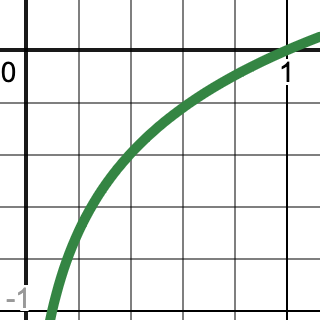
The closer it is to one (good), the loss becomes 0, and the closer to 0 the closer it gets to \(-\infty\).

2. The Spherical score

\(S_{sph}(q,y) = \frac{\sum{y_k\times q_k}}{\sqrt{\sum{q_k^2}}\})

Has the same goal as the log loss but has smoother gradient (no vertical asymptote at 0)

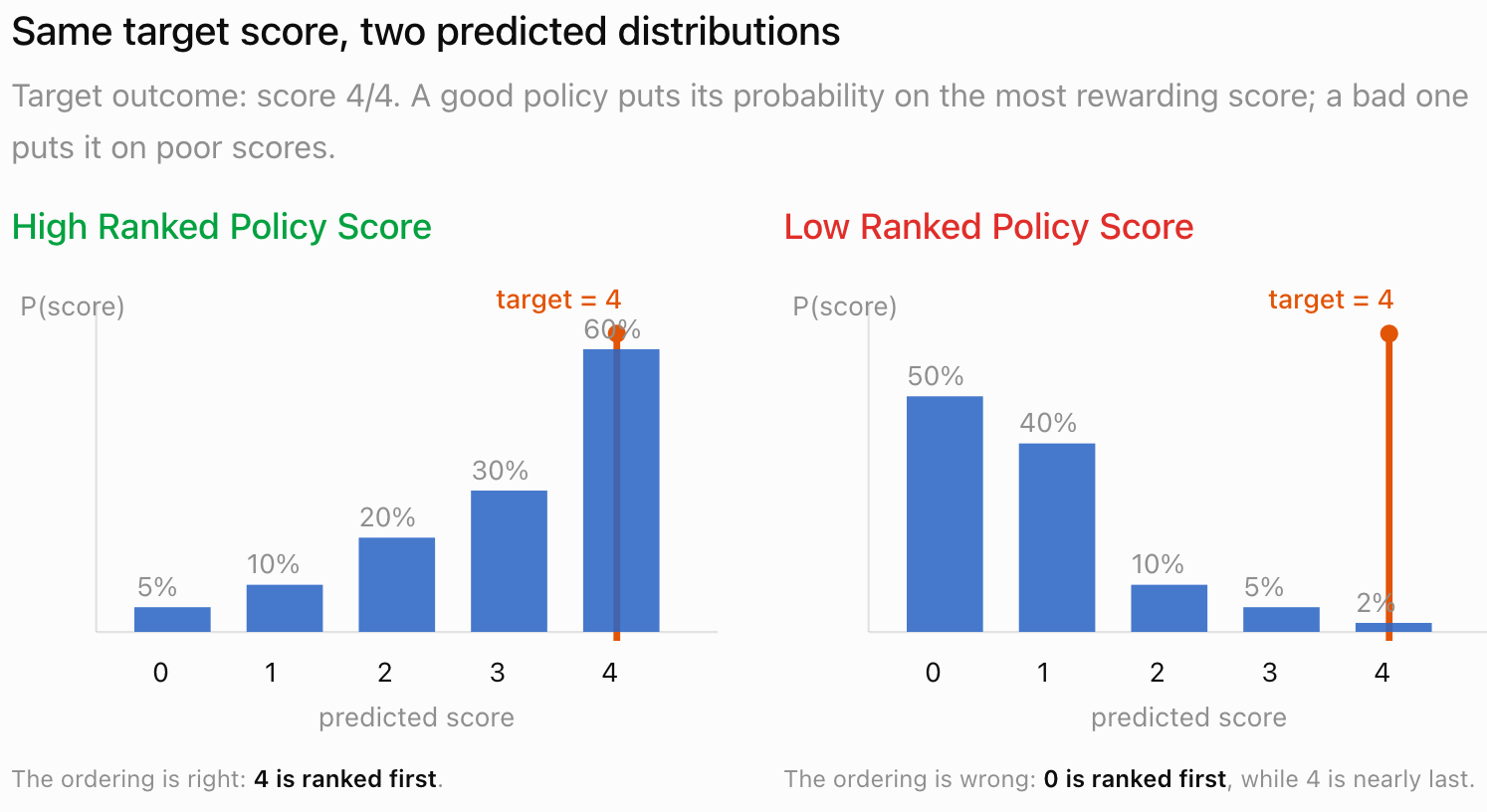
3. Ranked Probability Score

This one is only used for scoring questions where the order matters (if a < b < c, and the correct answer was c, then a will be highly penalized compared to b).

\(S_{rps}(q,y) = \frac{1}{K-1}\sum{(\text{CDF}_q(i) - \text{CDF}_y(i)})^2\)

Where CDF is the Cumulative Distribution Function: \( F_X(x) = \mathbb P(X \le x)\). So the term in the sum computes the distance between the two CDF.

The final reward becomes:

\( Reward(q,y) = S_{log}(q,y) + 0.5\times S_{sph}(q,y) - 1.0\times S_{rps}(q,y)\)

Then comes the RL part, inspired by GRPO (if you don't know about it, I highly advise you to read about it here, tldr: it is the reason why deepseek was able to make such good models with much less compute than OpenAI).

For each question, we sample G noisy candidates for the logits (\(c_i \sym \mathcal N(z, \sigma)\), we then compute the reward associated with those candidates and we compute the advantage

\(A = \frac{(r_noisy - mean(r))}{std(r) + 10^{-6}}\)

And from that we can compute the loss:

\(\mathcal L = -mean(A * log\_prob(z_{noisy} | z) )\)

This last expression forces to model to explore towards the candidates that had better results than the average (a positive advantage).

Confidence

The confidence formula is a bit different from the one from Jev

\(c = 1 - \frac{H(p)}{log(K)}\)

where H is the Shannon entropy defined by \(H(p) = -\sum{p_k\log(p_k)}\).

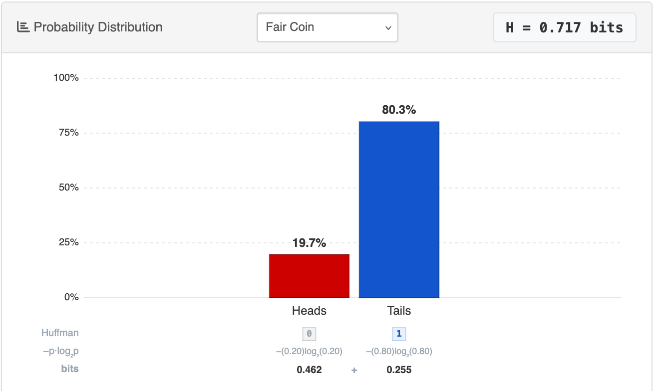
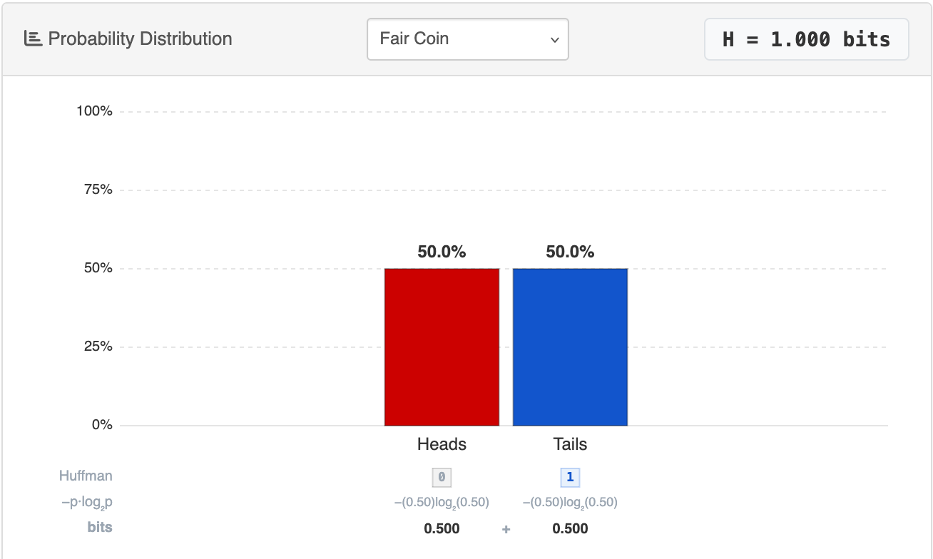
The Shannon entropy measures between 0 and 1 how unpredictable result is (how scattered is a distribution). For example figure A has an entropy lower than figure B.

Calibration

It is not over yet as you want to be sure that the confidence computed on your model outputs is close to the model accuracy (otherwise the confidence metric is useless). For that we use temperature finetuning. Temperature is a scalar that is used in the softmax layer (the one transforming logits into a probability distribution).

\(Softmax(z_i) = \frac{e^{\frac {z_i} {\tau}}}{\sum{e^{\frac {z_i} {\tau}}}}\)

Where \(\tau\) is the temperature, the lower it is the more skewed the probability distribution becomes (because of exponential properties). So in our case, having a low temperature will mean our model will be more confident.

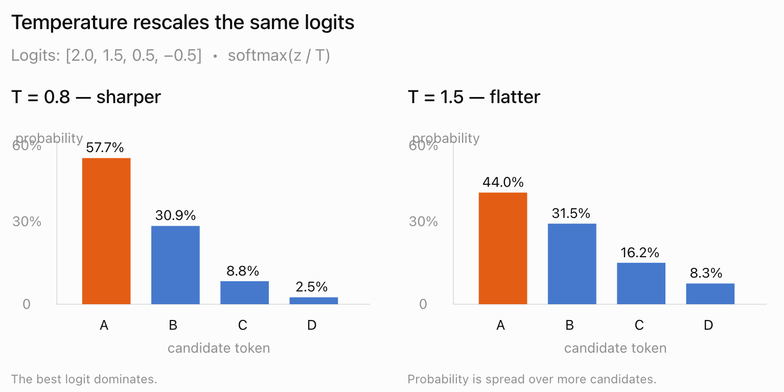
Then you evaluate your model and you find the temperature that minimizes the NLL (Negative Loss Likelihood). You can read more about calibration here.

Decoder (LLM) based (e.g. Kev)

Most of the most famous decision models are in this family (e.g Kev, Clef and allegedly Jev). The idea is similar to the previous one, take an existing model, take it's last hidden layer and do some stuff with it. But instead of training the whole LLM backbone, you only finetune it (with LoRA for example).

Architecture

We'll explain Kev's idea (as Clef is not open-source). The prompt format is a bit different that the one from Laya it is instead:

<state> Here is the state
<q> question instruction
<opt> option 1 </opt>
<opt> option 2 </opt>
<opt> option 3 </opt>
<decide>

Notice the <decide> token precisely at the end so it can attend at each previous token (because causal attention).

Once your LLM backbone has given you the last state \(z\) you get only the state of your </opt> tokens and your <decide> token. Then you perform the following:

\(l = \frac{Q(h_{opts})K(h_{decide})}{\tau\sqrt{d_p}}\)

Where \(h_{opts}\) and \(h_{decide}\) are the hidden states of the </opt> tokens and respectively the <decide> tokens. And \(d_p\) is the dimension of the pointer head (e.g. 256) and \(\tau\) the temperature.

Then your logits are given to a softmax and you can compute probabilities.

Loss function

Kev's loss function is a combination of Cross Entropy Loss, Brier loss, Focal loss, KL anchoring, and Permutation KL, RPS for scoring questions

Brier Loss

It's mean square error but for probabilities, so it is bounded unlike Cross Entropy Loss, so the model will first fix it's very uncorrect prediction then make it's distribution more precise with Brier.

\(\mathcal L_{Brier} = \sum{(p_i - t_i)^2}\)

Focal Loss

It's goal is to force the model to train harder (make the loss bigger) on difficult questions and easier (loss smaller) on easy ones. So it takes the already existing cross entropy loss as parameter.

\(\mathcal L_{focal} = -(1-p_y)^\gamma\log(p_y)\).

Where \(p_y\) is the guessed probability of the target (should be 1), and \(\gamma\) is an hyper-parameter.

KL anchoring

We want our decision model not to forget the knowledge of the LLM weights, for that we can use KL anchoring (see Kullback Leibler divergence, which measures the distance between two probability distributions). And we want our model not to go far away from the distrubtions of the base model (e.g. Qwen). For that we give Qwen the state+question in natural language like this:

Customer has requested a refund.

What action should we take?

A. Issue a refund
B. Offer store credit
C. Reject the request

Answer:

We then get the logits for A, B and C and perform a softmax to get the distribution.

Permutation KL

This one also uses the KL divergence but this time it penalizes the model for giving different answers at the same question but where options are not in the same order. For that we forward the model with two different orderings of the same question and then we compute:

\(\mathcal L_{perm} = \frac 1 2 (\mathcal D_{KL}(p || p^\pi) + \mathcal D_{KL}(p^\pi || p)\).

Notice that we average the two types of KL divergence the permuted one from the original and the original from the permuted. That's because KL divergence is asymmetric.`

Decoder based + transformer head (e.g. Clef)

Clef is basically a mix between Laya and Kev, take an existing LLM and give then do like Laya (a transformer decision head). Because Kev relies on having hidden outputs from the LLM to produce meaningful features for decision and also for predicting the next token.

Contrastive (e.g. CLM)

This method doesn't require to finetune the existing LLM, instead you get the last layers of the state+question, and the last layer for each option (candidate). Then you train a state encoder and a candidate encoder, and you compare the encoded state with encoded action with a dot product. That gives you the compatibility score => softmax => probabilities. The encoders have been trained with InfoNCE (which is a constrative method I don't know about, I'll update this section once I've trained a contrastive model).

You can read more about CLM here.

Other ideas

Don't train at all: use an existing LLM and just do a softmax on the logits of the available options keys (e.g. A, B, C, 1, 2, 3).

Conclusion

That's it, you now have a quite large vision on decision models, if anything is unclear please email me at matheoledev [at] gmail [dot] com.